Code
search_date <- "2023-01-06"
combined_data <- read_rds(here("others", "data", "raw_data", paste0(search_date, "_data.rds")))
project_crs <- "EPSG:4326"
rodent_locations <- combined_data$rodent %>%
  select(genus, species, latitude, longitude, number) %>%
  mutate(number = as.numeric(number)) %>%
  drop_na(number) %>%
  st_as_sf(coords = c("longitude", "latitude"), crs = project_crs) %>%
  group_by(geometry, species) %>%
  mutate(number = sum(number)) %>%
  ungroup() %>%
  distinct() %>%
  rowwise() %>%
  mutate(labels = HTML(paste0("Species: ", species, "<br>", "Number detected: ", number)))
pal <- colorFactor(diverging_hcl(n = length(sort(unique(rodent_locations$genus))), palette = "Berlin"),
                   domain = sort(unique(rodent_locations$genus)))
leaflet(data = rodent_locations) %>%
  addTiles() %>%
  addCircleMarkers(radius = ~ifelse(sqrt(number) == 0, 1, sqrt(number)),
                   color = ~pal(genus),
                   stroke = FALSE,
                   fillOpacity = 0.8,
                   clusterOptions = markerClusterOptions(spiderfyOnMaxZoom = TRUE,
                                                         spiderLegPolylineOptions = list(length = 6),
                                                         spiderfyDistanceMultiplier = 2),
                   label = ~labels,
                   popup = ~labels) %>%
  addLegend("bottomright", pal = pal, values = ~genus, title = "Host genus", opacity = 0.8)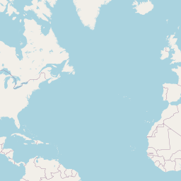

Host genus
ApodemusChaetodipus
Clethrionomys
Crocidura
Dasymys
Dipodomys
Dryomys
Grammomys
Graphiurus
Hybomys
Hylomyscus
Lemniscomys
Lophuromys
Malacomys
Mastomys
Micromys
Microtus
Mus
Myodes
Nannoyms
Neotoma
Onychomys
Peromyscus
Praomys
Rattus
Reithrodontomys
Sigmodon
Sorex
Spermophilus
Thomomys
Tscherskia
Uranomys
Urotrichus
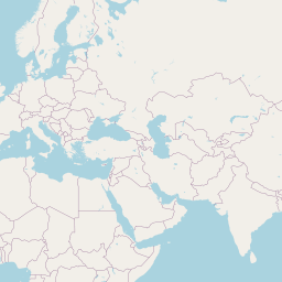
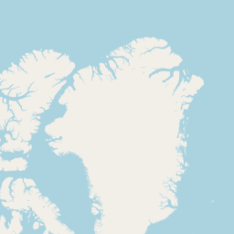
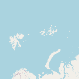
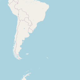
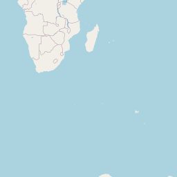
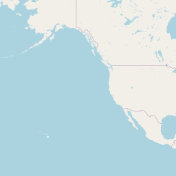
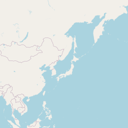
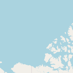
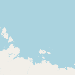
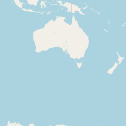
An interactive map displaying the location of detected small species in included studies. Selecting points will expand the number of data points at those coordinates. Point colour indicates small mammal genus with size of the point varying by the number of individuals detected. Hovering over a point or selecting it will show the species name, the number detected and the time period surveyed at the location. Data is currently shown for 9 studies.